Phillips Curve
Updated on 2023-08-29T11:57:38.744583Z
What is the Phillips curve?
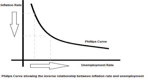
The relationship between the rate of inflation and the rate of unemployment is described by the Phillips curve. This was a significant finding in the field of macroeconomics by A.W.H Phillips. Phillips discovered a consistent inverse relationship, i.e. wage growth was slow when unemployment soared in the economy but aced when employment was higher.
Copyright © 2021 Kalkine Media
Summary
- The inverse relationship between the rate of inflation and the rate of unemployment is described by the Phillips curve.
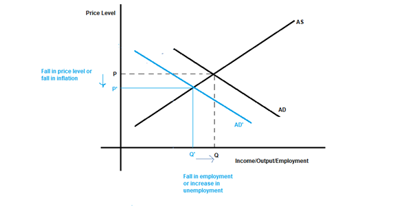
- Keynesian explanation of Phillip’s Curve states that, as the Aggregate Demand increases, price level and output in the economy increases and thus unemployment decreases.
- Monetarists had been dismissive of the Phillips curve trade-off claiming there is no trade-off in the long run due to the inelastic long run supply curve.
- Natural Rate of Unemployment (NAIRU) is the rate which the number of unemployed is equal to the number of jobs available in the labour market in a given period.
- In the long run any rate of inflation can persist at natural rate of unemployment.
Frequently Asked Questions (FAQs)
What are the origins of the concept of Phillips Curve?
Phillips used a scatter diagram to map annual wage inflation and unemployment rates in the United Kingdom from 1860 to 1957. Wage inflation and unemployment tended to have an inverse and stable relationship, according to the results.
The Phillips curve was created when economists substituted market inflation for wage inflation. When economists from other countries conducted similar studies, they discovered that their economies had very similar curves.
As the Aggregate Demand increases, price level and output in the economy increases. This also implies a decline in unemployment which is the Philips curve inverse relationship between inflation and unemployment. This is the Keynesian explanation of Phillip’s Curve.
Copyright © 2021 Kalkine Media
What is meant by the Collapse of Phillip's Curve?
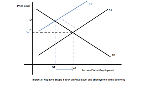
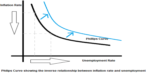
Around the 1960s, fiscal and monetary policy was being used to along the Philips curve as required. By the mid-1970s, it seemed that the Phillips Curve trade-off had vanished and that no consistent trend could be established. For any given unemployment rate, a variety of inflation rates may be used. Nations around the world, including the US, saw a simultaneous increase in inflation and unemployment. What actually happened was a shift in the Philips curve as opposed to the earlier movements along the Philips curve. This parallel increase in the two variables became known as stagflation where there was skyrocketing inflation along with very high unemployment. The stagflation back then was attributed to the mid-1970s oil crisis ushered in by the oil price hike by the OPEC cartel and to peoples’ expectations about inflation. Both these factors resulted in the shift of the aggregate supply curve and thus the Phillips curve. A leftward shift in AS curve would mean lower Output and employment at higher price levels as indicated in the simple AD-AS diagram below
Copyright © 2021 Kalkine Media
The impact of the above mentioned negative supply shock will get reflect on our previous Philips Curve diagram as shown below
Copyright © 2021 Kalkine Media
This phenomenon is called the Collapse of the Phillip's Curve.
What is the Monetarist view on the Phillip’s Curve?
Monetarists had been dismissive of the Phillips curve trade-off. They claim that because Long-Run Aggregate Supply is inelastic, there is no trade-off in the long run. Monetarists believe that if aggregate demand rises, employees would demand higher nominal wages. Basing their price forecast on the past year, They work more hours as they earn higher nominal salaries because they believe their real wages have risen. (their price forecasts are based on the previous year)
However, since the rise in AD triggers inflation, real wages remain unchanged. When they realise that real wages are unchanged from the previous year, they adjust their price forecasts, stop supplying extra labour, and real production returns to its previous level. As a result, unemployment remains stable, but inflation is higher. The Phillips curve moves upwards in the short term.
What is Natural Rate of Unemployment?
Friedman and Phelps were two American economists who proposed an explanation to the phenomenon that there is not one single Phillips curve, but multiple short-run Phillips Curves and one long-run Phillips Curve that prevails at the natural rate of unemployment (NAIRU). NAIRU is the rate at which the number of unemployed is equal to the number of jobs available in the labour market in a given period. In the long run, there isn’t thus a trade-off between unemployment and inflation. Instead, the long-run Phillips curve is a vertical straight line. The existing unemployment is due to structural and frictional reasons thus; full employment is deemed to exist. The expectations about future inflation rate also have a role to play in this phenomenon. Friedman proposed the theory of adaptive expectations. As per this theory, people set their expectations about inflation based on the current rates and the rates prevalent in the previous period, and they change their expectations only then the actuals are deviant from the expected rate. There may thus be a trade-off between inflation and unemployment in the short run but not in the long run.
What is the Long Run Phillips Curve?
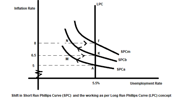
Copyright © 2021 Kalkine Media
The diagram above uses hypothetical numbers to explain the phenomenon of the Long Run Phillips Curve. As per A.W. Phillips, we can explain the movement A to M on SPCa- initially at point A, unemployment is at 5% and inflation is at 5%. Due to a factor like expansionary monetary policy, inflation in the economy rises and unemployment falls, and there is a movement to point M. According to Friedman and the supporters of NAIRU theory, M is not a stable point. This is because workers will realise gradually that due to the risen inflation levels, their real incomes have fallen. As a result, worker will demand higher nominal wages so as to restore their previous purchasing power or real income. This will result in employers losing the earlier earned profits, which had induced them to increase production and thus curb the problem of unemployment at levels corresponding to M. As a result, cost-cutting begins, and employment will fall in the economy till it reaches back 5.5% from point M to point K. Once this inflation rate of 6.5% is reached, the workers will expect the 6.5% to continue in future. Thus there is a shift up from SPCa to SPCb, and unemployment is at 5.5% and the inflation rate at 6.5%. Thus we see that as per natural theorists, the movement along an SPC is only a short-run phenomenon. In the long run, when nominal wages adapted to the risen inflation levels and unemployment is back to the NAIRU level (5.5% here), a new SPC is formed at the new higher inflation level. This process of improved employment followed by inflation and increased unemployment will persist as there is a movement from point K to N and then from N to F and to further higher levels to inflation. Joining the points, A, K and F will help us arrive at the long-run Phillips Curve (LPC), which is a vertical line parallel to the y axis. Showing no trade-off exists between unemployment and inflation in the long run. It thus follows from the above explanation that any rate of inflation can persist at the natural rate of unemployment.